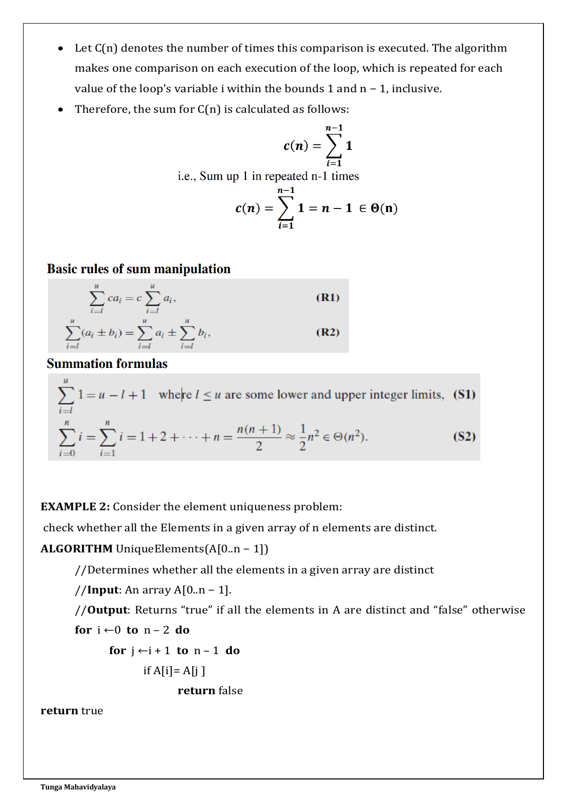
Σ → closed form M(n) → recurrence Python → practice
All 12 source pages9 interactive animations8 runnable Python programsMobile friendly
Your complete notes, with interactive explanations alongside them.
Every page’s text, original equations and diagrams are retained. Original wording includes source inconsistencies; separate green panels explain them. Open each original page to compare with the readable text. All animation controls are manual unless you choose Play.
Source: Unit 2 Asymptotic and Brute force · Tunga Mahavidyalaya · supplied by you.
DAA · UNIT 2 · 01
Describe growth with a precise bound.
ORIGINAL NOTES · PAGE 1 OF 12
Tunga Mahavidyalaya
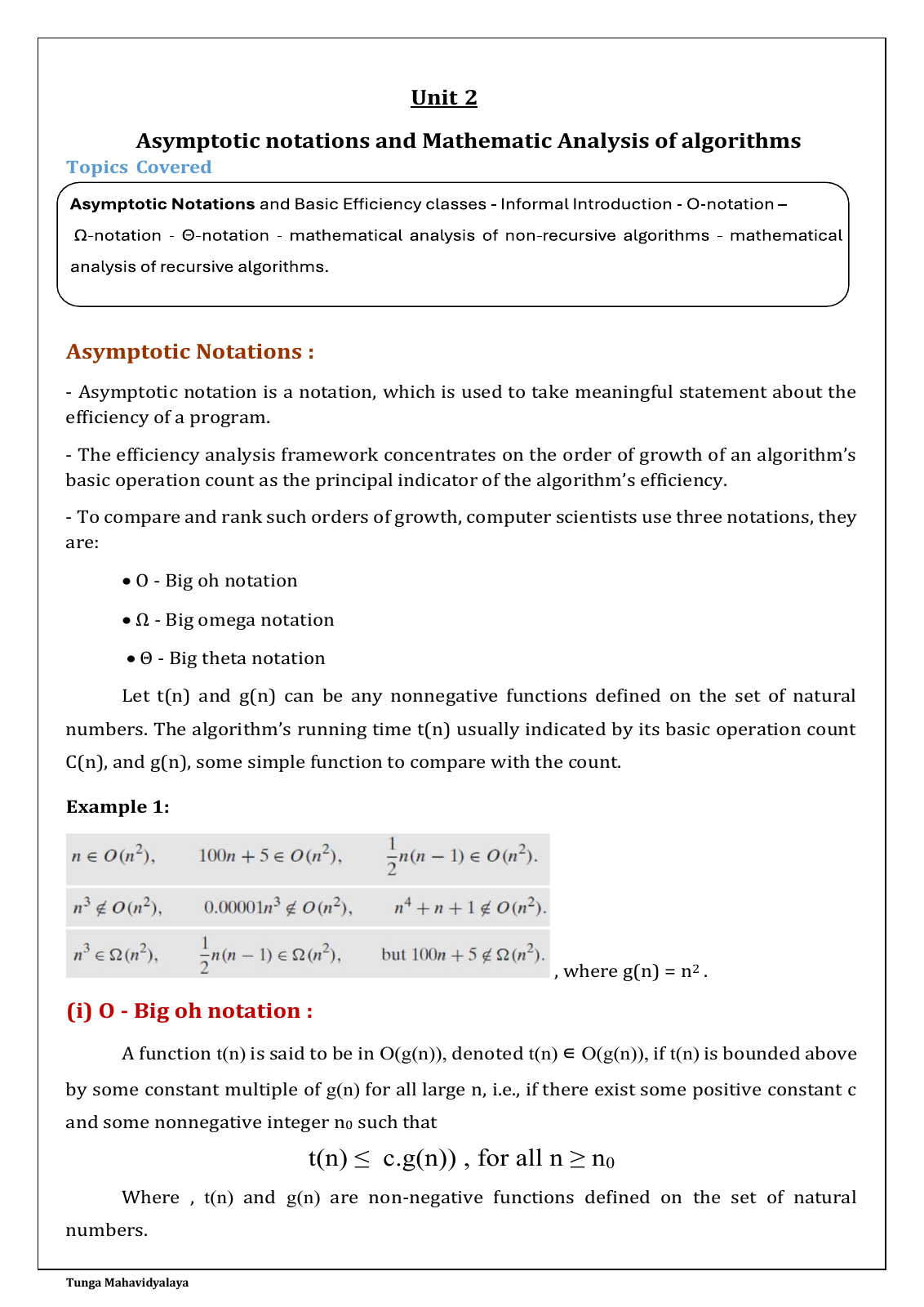
Unit 2
Asymptotic notations and Mathematic Analysis of algorithms
Topics Covered
Asymptotic Notations :
- Asymptotic notation is a notation, which is used to take meaningful statement about the
efficiency of a program.
- The efficiency analysis framework concentrates on the order of growth of an algorithm’s
basic operation count as the principal indicator of the algorithm’s efficiency.
- To compare and rank such orders of growth, computer scientists use three notations, they
are:
• O - Big oh notation
• Ω - Big omega notation
• Θ - Big theta notation
Let t(n) and g(n) can be any nonnegative functions defined on the set of natural
numbers. The algorithm’s running time t(n) usually indicated by its basic operation count
C(n), and g(n), some simple function to compare with the count.
Example 1:
, where g(n) = n2 .
(i) O - Big oh notation :
A function t(n) is said to be in O(g(n)), denoted t(n) ∊ O(g(n)), if t(n) is bounded above
by some constant multiple of g(n) for all large n, i.e., if there exist some positive constant c
and some nonnegative integer n0 such that
t(n) ≤ c.g(n)) , for all n ≥ n0
Where , t(n) and g(n) are non -negative functions defined on the set of natural
numbers.
Text from equations / figures on this page
Topics Covered: Asymptotic Notations and Basic Efficiency classes - Informal Introduction - O-notation – Ω-notation - Θ-notation - mathematical analysis of non-recursive algorithms - mathematical analysis of recursive algorithms.
Example 1 (equations printed as an image):
n ∈ O(n²), 100n + 5 ∈ O(n²), ½n(n − 1) ∈ O(n²).
n³ ∉ O(n²), 0.00001n³ ∉ O(n²), n⁴ + n + 1 ∉ O(n²).
n³ ∈ Ω(n²), ½n(n − 1) ∈ Ω(n²), but 100n + 5 ∉ Ω(n²).
Tunga Mahavidyalaya
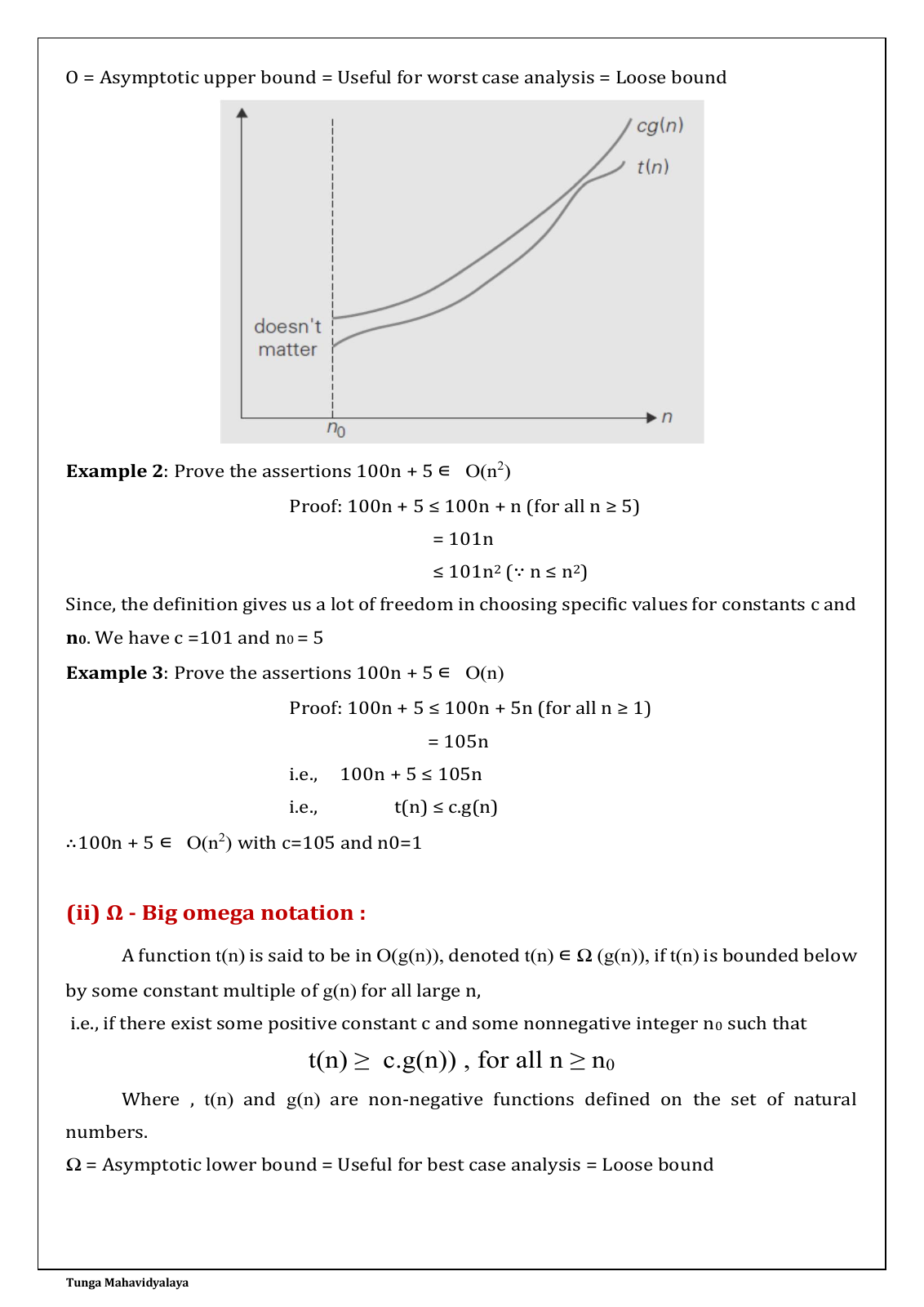
O = Asymptotic upper bound = Useful for worst case analysis = Loose bound
Example 2: Prove the assertions 100n + 5 ∊ O(n2)
Proof: 100n + 5 ≤ 100n + n (for all n ≥ 5)
= 101n
≤ 101n2 (∵ n ≤ n2)
Since, the definition gives us a lot of freedom in choosing specific values for constants c and
n0. We have c =101 and n0 = 5
Example 3: Prove the assertions 100n + 5 ∊ O(n)
Proof: 100n + 5 ≤ 100n + 5n (for all n ≥ 1)
= 105n
i.e., 100n + 5 ≤ 105n
i.e., t(n) ≤ c.g(n)
∴100n + 5 ∊ O(n2) with c=105 and n0=1
(ii) Ω - Big omega notation :
A function t(n) is said to be in O(g(n)), denoted t(n) ∊ Ω (g(n)), if t(n) is bounded below
by some constant multiple of g(n) for all large n,
i.e., if there exist some positive constant c and some nonnegative integer n 0 such that
t(n) ≥ c.g(n)) , for all n ≥ n0
Where , t(n) and g(n) are non -negative functions defined on the set of natural
numbers.
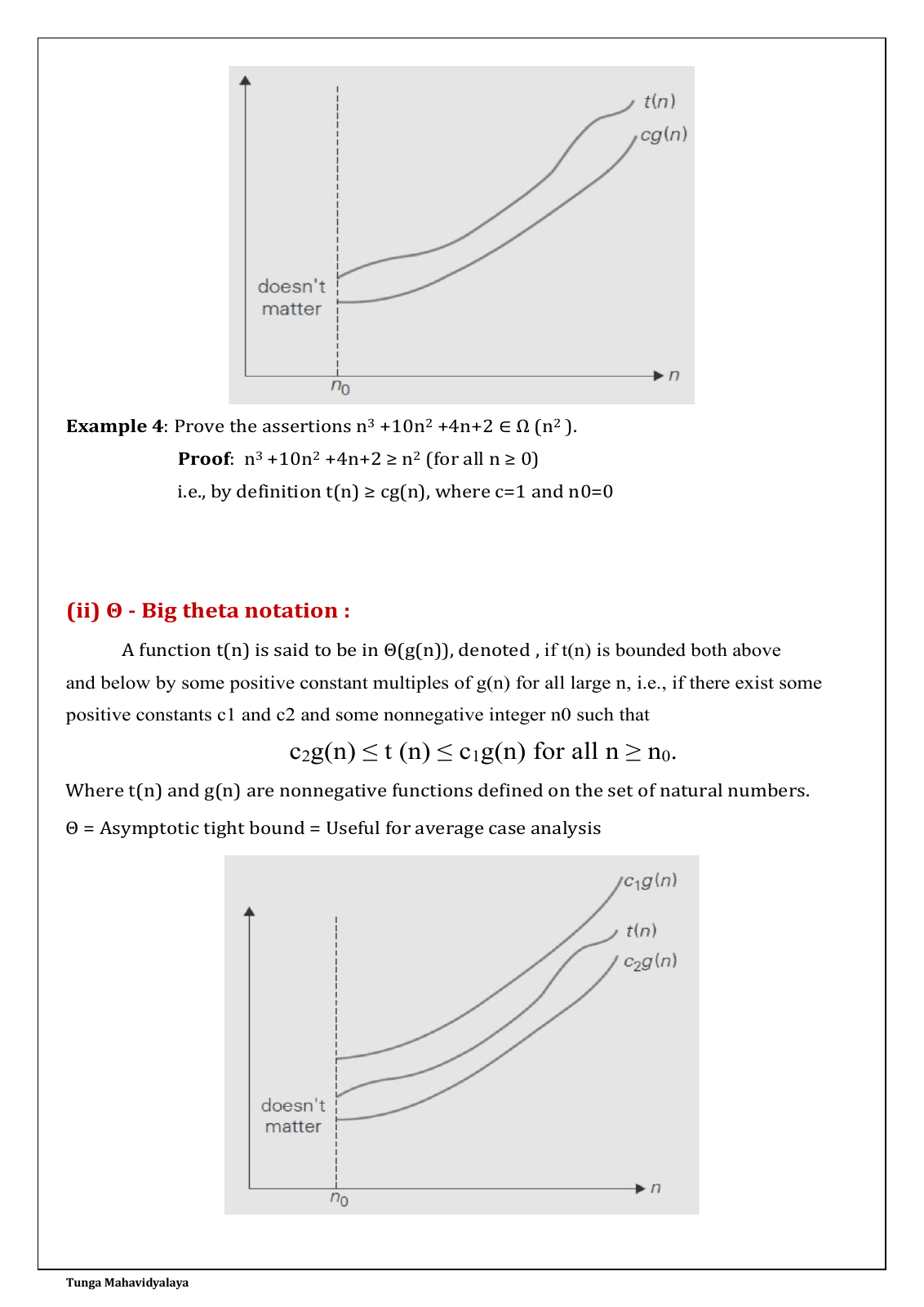
Ω = Asymptotic lower bound = Useful for best case analysis = Loose bound
Text from equations / figures on this page
Big O graph: t(n) is below cg(n) for n ≥ n₀. A vertical dashed line marks n₀. The earlier region is labelled “doesn’t matter”.
Tunga Mahavidyalaya
Example 4: Prove the assertions n3 +10n2 +4n+2 ∈ Ω (n2 ).
Proof: n3 +10n2 +4n+2 ≥ n2 (for all n ≥ 0)
i.e., by definition t(n) ≥ cg(n), where c=1 and n0=0
(ii) Θ - Big theta notation :
A function t(n) is said to be in Θ(g(n)), denoted , if t(n) is bounded both above
and below by some positive constant multiples of g(n) for all large n, i.e., if there exist some
positive constants c1 and c2 and some nonnegative integer n0 such that
c2g(n) ≤ t (n) ≤ c1g(n) for all n ≥ n0.
Where t(n) and g(n) are nonnegative functions defined on the set of natural numbers.
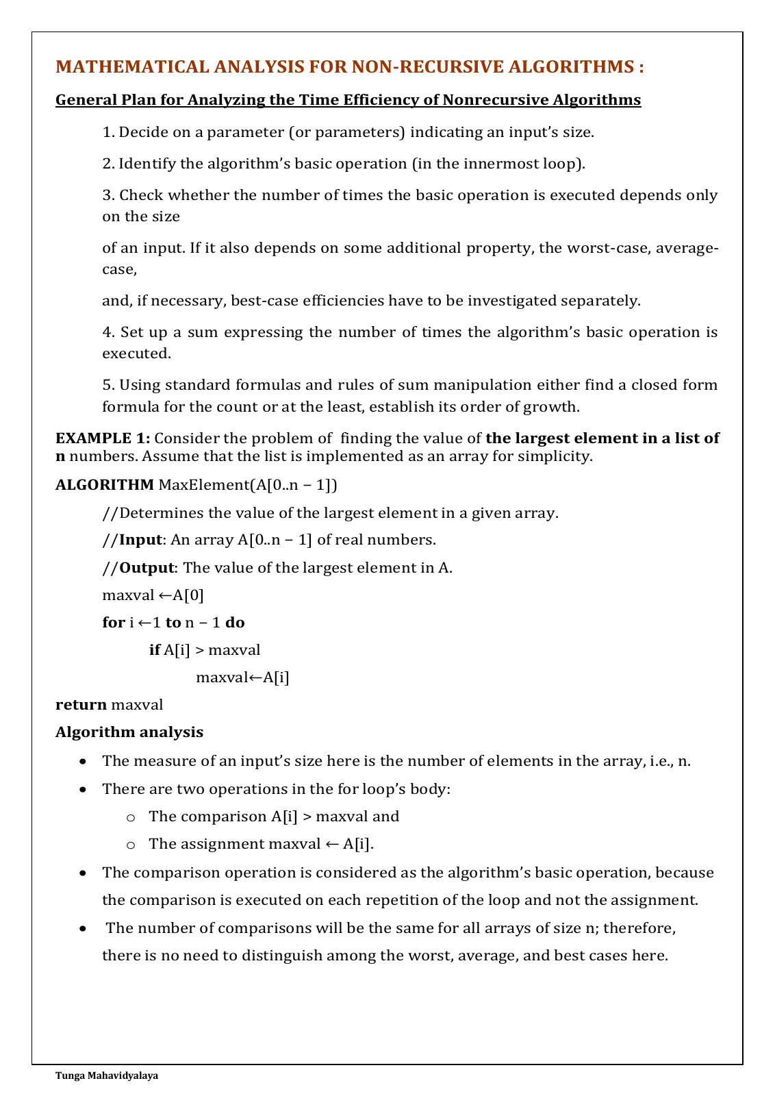
Θ = Asymptotic tight bound = Useful for average case analysis
Text from equations / figures on this page
Big Ω graph: t(n) is above cg(n) for n ≥ n₀.
Big Θ graph: c₂g(n) ≤ t(n) ≤ c₁g(n) for n ≥ n₀. The earlier region is labelled “doesn’t matter”.
Read the original definitions above exactly as supplied. O gives an eventual upper bound, Ω an eventual lower bound, and Θ both. These notations can describe any specified best-, average- or worst-case count; they are not restricted to one case each. O can be tight or loose. A graph over finitely many values illustrates a claim but cannot prove a bound for every sufficiently large n. The proof is the inequality and constants.
Notation
Condition for all n ≥ n₀
Example
O(g(n))
t(n) ≤ c g(n), c > 0
100n + 5 ≤ 105n for n ≥ 1.
Ω(g(n))
t(n) ≥ c g(n), c > 0
100n + 5 ≥ 100n for n ≥ 1.
Θ(g(n))
c₂g(n) ≤ t(n) ≤ c₁g(n), c₁,c₂ > 0
100n ≤ 100n + 5 ≤ 105n for n ≥ 1.
ADDED INTERACTIVE EXPLANATION
Watch upper, lower and tight bounds
Follow t(n) = 100n + 5 against g(n) = n. The constants are fixed: upper 105, lower 100, threshold n₀ = 1. Curves are close together; read the values as well as the graph.
Enable JavaScript for the animation. The complete notes and programs remain readable.
Added explanation · Python lab
Source clarification: page 2 Example 3 proves the linear bound O(n), although its final line prints O(n²). The Ω definition on page 2 begins with O(g(n)); its heading, lower-bound inequality and denoted membership identify Ω. These original lines are retained. Page 3 labels Θ “(ii)” again. We explain these slips separately.
O, Ω and Θ: inspect a linear boundmain.py
# Finite samples illustrate a bound; the algebra establishes it for all n >= 1.
# 100*n <= 100*n + 5 <= 105*n, since 5 <= 5*n.
limit = int(input())
if not 1 <= limit <= 30:
raise ValueError("Choose a sample limit from 1 to 30")
print("n | lower | t(n) | upper")
for n in range(1, limit + 1):
lower, actual, upper = 100 * n, 100 * n + 5, 105 * n
print(n, lower, actual, upper, sep=" | ")
Tunga Mahavidyalaya
MATHEMATICAL ANALYSIS FOR NON-RECURSIVE ALGORITHMS :
General Plan for Analyzing the Time Efficiency of Nonrecursive Algorithms
1. Decide on a parameter (or parameters) indicating an input’s size.
2. Identify the algorithm’s basic operation (in the innermost loop).
3. Check whether the number of times the basic operation is executed depends only
on the size
of an input. If it also depends on some additional property, the worst -case, average-
case,
and, if necessary, best-case efficiencies have to be investigated separately.
4. Set up a sum expressing the number of times the algorithm’s basic operation is
executed.
5. Using standard formulas and rules of sum manipulation either find a closed form
formula for the count or at the least, establish its order of growth.
EXAMPLE 1: Consider the problem of finding the value of the largest element in a list of
n numbers. Assume that the list is implemented as an array for simplicity.
ALGORITHM MaxElement(A[0..n − 1])
//Determines the value of the largest element in a given array.
//Input: An array A[0..n − 1] of real numbers.
//Output: The value of the largest element in A.
maxval ←A[0]
for i ←1 to n − 1 do
if A[i] > maxval
maxval←A[i]
return maxval
Algorithm analysis
• The measure of an input’s size here is the number of elements in the array, i.e., n.
• There are two operations in the for loop’s body:
o The comparison A[i] > maxval and
o The assignment maxval ← A[i].
• The comparison operation is considered as the algorithm’s basic operation, because
the comparison is executed on each repetition of the loop and not the assignment.
• The number of comparisons will be the same for all arrays of size n; therefore,
there is no need to distinguish among the worst, average, and best cases here.
Tunga Mahavidyalaya
• Let C(n) denotes the number of times this comparison is executed. The algorithm
makes one comparison on each execution of the loop, which is repeated for each
value of the loop’s variable i within the bounds 1 and n − 1, inclusive.
• Therefore, the sum for C(n) is calculated as follows:
EXAMPLE 2: Consider the element uniqueness problem:
check whether all the Elements in a given array of n elements are distinct.
ALGORITHM UniqueElements(A[0..n − 1])
//Determines whether all the elements in a given array are distinct
//Input: An array A[0..n − 1].
//Output: Returns “true” if all the elements in A are distinct and “false” otherwise
for i ←0 to n – 2 do
for j ←i + 1 to n – 1 do
if A[i]= A[j ]
return false
return true
Text from equations / figures on this page
C(n) = Σ(i = 1…n − 1) 1
i.e., Sum up 1 in repeated n − 1 times
C(n) = Σ(i = 1…n − 1) 1 = n − 1 ∈ Θ(n)
Basic rules of sum manipulation
R1: Σ(i = l…u) c aᵢ = c Σ(i = l…u) aᵢ
R2: Σ(i = l…u) (aᵢ ± bᵢ) = Σ(i = l…u) aᵢ ± Σ(i = l…u) bᵢ
Summation formulas
S1: Σ(i = l…u) 1 = u − l + 1,
where l ≤ u are some lower and upper integer limits
S2: Σ(i = 0…n) i = Σ(i = 1…n) i = 1 + 2 + … + n
= n(n + 1)/2 ≈ ½n² ∈ Θ(n²)
For MaxElement the array must be nonempty. A list of one element performs zero comparisons. Every nonempty input of length n performs n − 1 comparisons, although the number of assignments varies. In Python, range(1, len(values)) includes indices 1 through n − 1. Θ(n) describes growth as n increases; it does not mean n comparisons exactly.
ADDED INTERACTIVE EXPLANATION
Inspect every value and maintain the maximum
The first element initializes maxval. Only later elements require a comparison. Try descending, ascending and repeated values: the comparison count stays n − 1.
Enable JavaScript for the animation. The complete notes and programs remain readable.
Largest element: exactly n − 1 comparisonsmain.py
def max_element(values):
if not values:
raise ValueError("The array must be nonempty")
maximum, comparisons = values[0], 0
for i in range(1, len(values)):
comparisons += 1
if values[i] > maximum:
maximum = values[i]
return maximum, comparisons
values = list(map(int, input().split()))
maximum, comparisons = max_element(values)
print("Maximum =", maximum)
print("Comparisons =", comparisons)
Row i contributes i tiles. The completed triangle has n(n + 1)/2 tiles. S1 counts the integer indices in an inclusive interval; R1 moves a constant outside a sum.
Enable JavaScript for the animation. The complete notes and programs remain readable.
Added explanation · Python lab
For n = 5, 1 + 2 + 3 + 4 + 5 = 15. For a constant summand, Σ(i = 1…n − 1) 1 = (n − 1) − 1 + 1 = n − 1. Use an empty sum of zero when n = 1; the printed S1 formula assumes the lower limit does not exceed the upper limit.
DAA · UNIT 2 · 03
Compare pairs. Stop at the first duplicate.
ORIGINAL NOTES · PAGE 6 OF 12
Tunga Mahavidyalaya
Algorithm analysis
• The natural measure of the input’s size here is again n.
• Since the innermost loop contains a single operation, we should consider it as the
algorithm’s basic operation.
• The number of element comparisons depends not only on n but also on whether
there are equal elements in the array and, if there are, which array positions they
occupy. We will limit our investigation to the worst case only.
• One comparison is made for each repetition of the innermost loop, i.e., for each
value of the loop variable j between its limits i + 1 and n − 1; this is repeated for
each value of the outer loop, i.e., for each value of the loop variable i between its
limits 0 and n − 2.
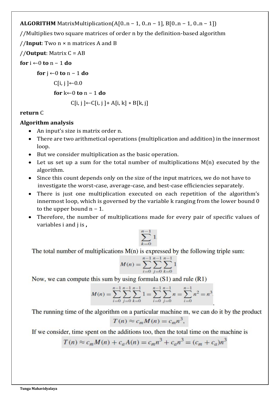
EXAMPLE 3: Consider matrix multiplication. Given two n × n matrices A and B, find the
time efficiency of the definition-based algorithm for computing their product
C = AB. By definition, C is an n × n matrix whose elements are computed as the scalar (dot)
products of the rows of matrix A and the columns of matrix B:
where C[i, j ]= A[i, 0]B[0, j]+ . . . + A[i, k]B[k, j]+ . . . + A[i, n − 1]B[n − 1, j] for every pair of
indices 0 ≤ i, j ≤ n − 1.
Text from equations / figures on this page
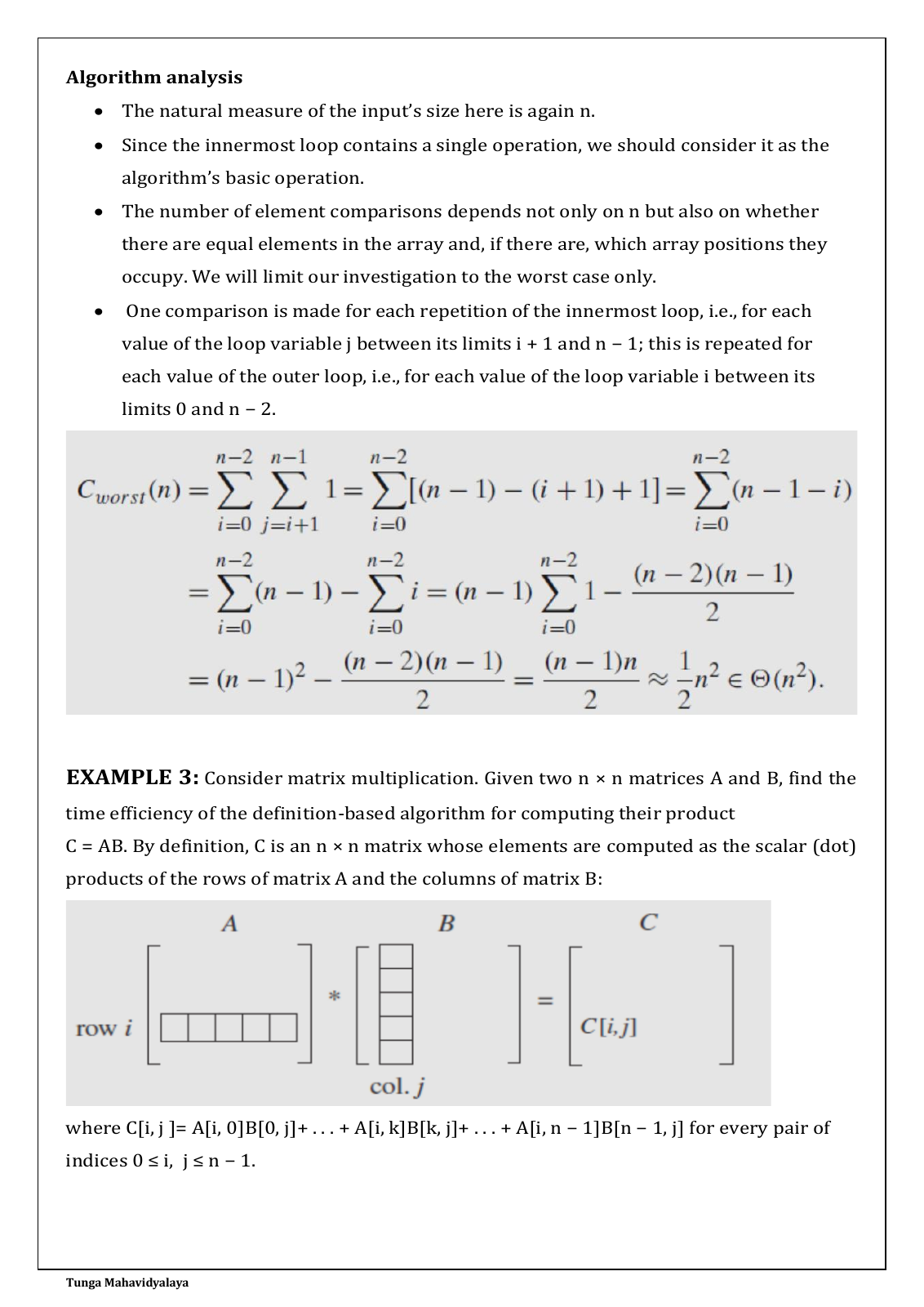
Cworst(n) = Σ(i = 0…n − 2) Σ(j = i + 1…n − 1) 1
= Σ(i = 0…n − 2) [(n − 1) − (i + 1) + 1]
= Σ(i = 0…n − 2) (n − 1 − i)
= Σ(i = 0…n − 2) (n − 1) − Σ(i = 0…n − 2) i
= (n − 1) Σ(i = 0…n − 2) 1 − (n − 2)(n − 1)/2
= (n − 1)² − (n − 2)(n − 1)/2
= (n − 1)n/2 ≈ ½n² ∈ Θ(n²)
Matrix diagram: row i of A is multiplied with column j of B to obtain element C[i,j] of C = AB.
Only pairs i < j are checked. Try 3 3 5 for immediate failure, or 3 1 5 7 3 for a later duplicate. Change the input to restart the trace.
Enable JavaScript for the animation. The complete notes and programs remain readable.
Added explanation · Python lab
For five distinct values the pair count is 4 + 3 + 2 + 1 = 10. The worst case checks all n(n − 1)/2 pairs, including a duplicate discovered on the final pair. For n ≥ 2 the best case takes one comparison when the first pair matches. Empty and singleton lists are distinct without comparisons; the animation uses nonempty inputs. This brute-force implementation uses a constant number of auxiliary variables. A set-based approach is a different algorithm and is intentionally not substituted for the source pseudocode.
Element uniqueness: compare every required pairmain.py
def unique_elements(values):
comparisons = 0
for i in range(len(values) - 1):
for j in range(i + 1, len(values)):
comparisons += 1
if values[i] == values[j]:
return False, comparisons
return True, comparisons
values = list(map(int, input().split()))
unique, comparisons = unique_elements(values)
print("All distinct =", unique)
print("Comparisons =", comparisons)
n = len(values)
print("Worst-case pair count =", n * (n - 1) // 2)
Tunga Mahavidyalaya
ALGORITHM MatrixMultiplication(A[0..n − 1, 0..n − 1], B[0..n − 1, 0..n − 1])
//Multiplies two square matrices of order n by the definition-based algorithm
//Input: Two n × n matrices A and B
//Output: Matrix C = AB
for i ←0 to n − 1 do
for j ←0 to n − 1 do
C[i, j ]←0.0
for k←0 to n − 1 do
C[i, j ]←C[i, j ]+ A[i, k] ∗ B[k, j]
return C
Algorithm analysis
• An input’s size is matrix order n.
• There are two arithmetical operations (multiplication and addition) in the innermost
loop.
• But we consider multiplication as the basic operation.
• Let us set up a sum for the total number of multiplications M(n) executed by the
algorithm.
• Since this count depends only on the size of the input matrices, we do not have to
investigate the worst-case, average-case, and best-case efficiencies separately.
• There is just one multiplication executed on each repetition of the algorithm’s
innermost loop, which is governed by the variable k ranging from the lower bound 0
to the upper bound n − 1.
• Therefore, the number of multiplications made for every pair of specific values of
variables i and j is ,
Text from equations / figures on this page
For each specific pair i and j: Σ(k = 0…n − 1) 1
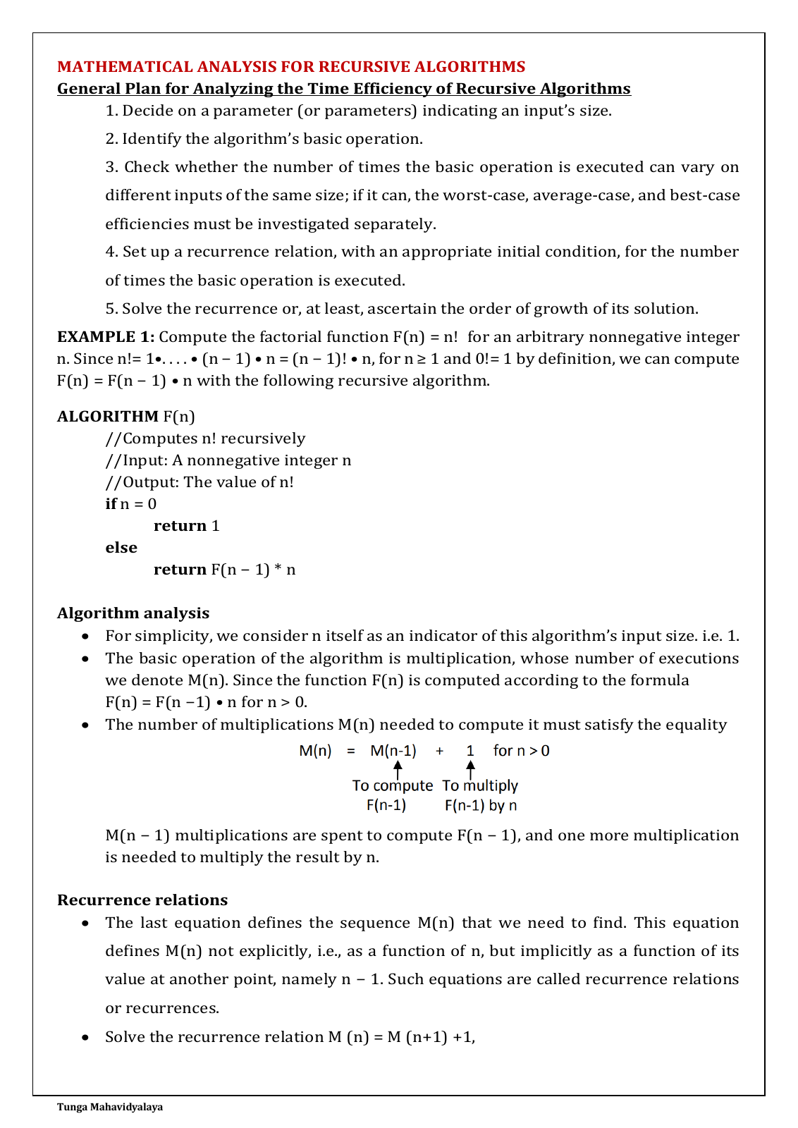
The total number of multiplications M(n) is expressed by the following triple sum:
M(n) = Σ(i = 0…n − 1) Σ(j = 0…n − 1) Σ(k = 0…n − 1) 1
Now, we can compute this sum by using formula (S1) and rule (R1)
M(n) = Σ(i = 0…n − 1) Σ(j = 0…n − 1) Σ(k = 0…n − 1) 1
= Σ(i = 0…n − 1) Σ(j = 0…n − 1) n
= Σ(i = 0…n − 1) n² = n³.
The running time of the algorithm on a particular machine m, we can do it by the product
T(n) ≈ cₘ M(n) = cₘ n³.
If we consider time spent on the additions too, then the total time on the machine is
T(n) ≈ cₘ M(n) + cₐ A(n) = cₘ n³ + cₐ n³ = (cₘ + cₐ)n³.
Each step multiplies one A[i,k] by one B[k,j], then adds the product into C[i,j]. Values must be integers from −20 to 20. The highlighted operands show why rows meet columns.
Enable JavaScript for the animation. The complete notes and programs remain readable.
Added explanation · Python lab
With A = [[1,2],[3,4]] and B = [[5,6],[7,8]], C[0,0] = 1×5 + 2×7 = 19. The complete product is [[19,22],[43,50]]. Two outer loops choose n² output cells and the inner loop performs n multiplications per cell: n³ in total. This exact algorithm also performs n³ additions, including additions into the initial zero. The output matrix occupies Θ(n²) storage; excluding that output, the loop variables require Θ(1) auxiliary storage.
def matrix_multiply(a, b):
n = len(a)
if n == 0 or len(b) != n or any(len(row) != n for row in a + b):
raise ValueError("Two nonempty square matrices of the same order are required")
c = [[0 for _ in range(n)] for _ in range(n)]
multiplications = 0
for i in range(n):
for j in range(n):
for k in range(n):
c[i][j] += a[i][k] * b[k][j]
multiplications += 1
return c, multiplications
n = int(input())
if not 1 <= n <= 20:
raise ValueError("Choose an order from 1 to 20 for this lab")
a = [list(map(int, input().split())) for _ in range(n)]
b = [list(map(int, input().split())) for _ in range(n)]
product, count = matrix_multiply(a, b)
print("Product:")
for row in product:
print(*row)
print("Multiplications =", count)
Tunga Mahavidyalaya
MATHEMATICAL ANALYSIS FOR RECURSIVE ALGORITHMS
General Plan for Analyzing the Time Efficiency of Recursive Algorithms
1. Decide on a parameter (or parameters) indicating an input’s size.
2. Identify the algorithm’s basic operation.
3. Check whether the number of times the basic operation is executed can vary on
different inputs of the same size; if it can, the worst-case, average-case, and best-case
efficiencies must be investigated separately.
4. Set up a recurrence relation, with an appropriate initial condition, for the number
of times the basic operation is executed.
5. Solve the recurrence or, at least, ascertain the order of growth of its solution.
EXAMPLE 1: Compute the factorial function F(n) = n! for an arbitrary nonnegative integer
n. Since n!= 1•. . . . • (n − 1) • n = (n − 1)! • n, for n ≥ 1 and 0!= 1 by definition, we can compute
F(n) = F(n − 1) • n with the following recursive algorithm.
ALGORITHM F(n)
//Computes n! recursively
//Input: A nonnegative integer n
//Output: The value of n!
if n = 0
return 1
else
return F(n − 1) * n
Algorithm analysis
• For simplicity, we consider n itself as an indicator of this algorithm’s input size. i.e. 1.
• The basic operation of the algorithm is multiplication, whose number of executions
we denote M(n). Since the function F(n) is computed according to the formula
F(n) = F(n −1) • n for n > 0.
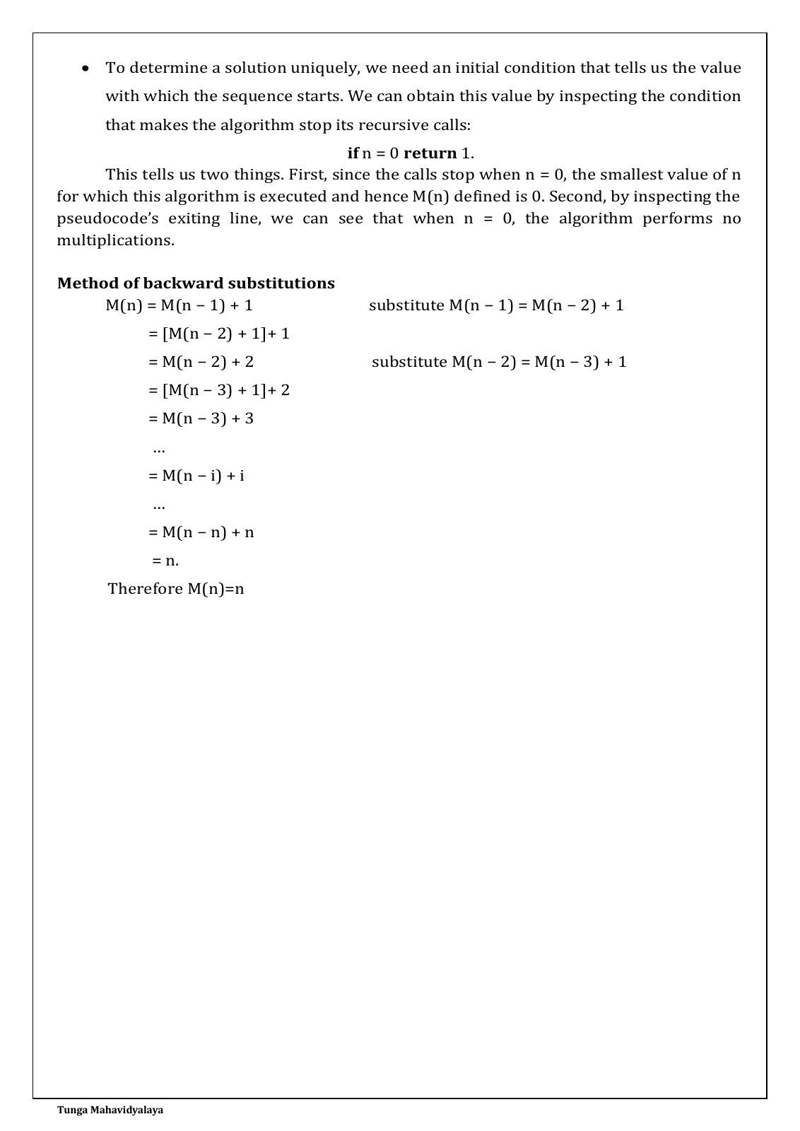
• The number of multiplications M(n) needed to compute it must satisfy the equality
M(n − 1) multiplications are spent to compute F(n − 1), and one more multiplication
is needed to multiply the result by n.
Recurrence relations
• The last equation defines the sequence M(n) that we need to find. This equation
defines M(n) not explicitly, i.e., as a function of n, but implicitly as a function of its
value at another point, namely n − 1. Such equations are called recurrence relations
or recurrences.
• Solve the recurrence relation M (n) = M (n+1) +1,
Text from equations / figures on this page
M(n) = M(n − 1) + 1 for n > 0
M(n − 1): To compute F(n − 1)
+1: To multiply F(n − 1) by n
Tunga Mahavidyalaya
• To determine a solution uniquely, we need an initial condition that tells us the value
with which the sequence starts. We can obtain this value by inspecting the condition
that makes the algorithm stop its recursive calls:
if n = 0 return 1.
This tells us two things. First, since the calls stop when n = 0, the smallest value of n
for which this algorithm is executed and hence M(n) defined is 0. Second, by inspecting the
pseudocode’s exiting line, we can see that when n = 0, the algorithm performs no
multiplications.
Method of backward substitutions
M(n) = M(n − 1) + 1 substitute M(n − 1) = M(n − 2) + 1
= [M(n − 2) + 1]+ 1
= M(n − 2) + 2 substitute M(n − 2) = M(n − 3) + 1
= [M(n − 3) + 1]+ 2
= M(n − 3) + 3
…
= M(n − i) + i
…
= M(n − n) + n
= n.
Therefore M(n)=n
Descend to F(0), return 1, then multiply while unwinding. Count the multiplication steps separately from the calls. No multiplication happens at the base case.
Enable JavaScript for the animation. The complete notes and programs remain readable.
ADDED INTERACTIVE EXPLANATION
Expand the recurrence backwards
Replace M(n − 1) by M(n − 2) + 1 repeatedly. Finish at the initial condition M(0) = 0.
Enable JavaScript for the animation. The complete notes and programs remain readable.
Added explanation · Python lab
The base case supplies M(0) = 0. For n > 0, M(n) = M(n − 1) + 1, hence M(n) = M(n − i) + i. Set i = n to obtain M(n) = M(0) + n = n. There are n + 1 function calls, n multiplications, and Θ(n) stack depth. The output value is n!, but this does not give the algorithm Θ(n!) time. The count assumes unit-cost multiplication; Python big-integer costs increase with operand size. The sample limits n to 100 to keep the recursion demonstration manageable.
Added explanation · Python lab
Source clarification: page 8’s last line prints M(n) = M(n+1) + 1. The algorithm, preceding diagram and page 9’s substitutions use n − 1. That printed line remains in the original notes above; the runnable program follows the algorithm.
Recursive factorial: count multiplications and callsmain.py
def factorial(n):
if n == 0:
return 1, 0, 1
value, multiplications, calls = factorial(n - 1)
return value * n, multiplications + 1, calls + 1
n = int(input())
if not 0 <= n <= 100:
raise ValueError("Choose n from 0 to 100 for this recursion demonstration")
value, multiplications, calls = factorial(n)
print("Factorial =", value)
print("Multiplications =", multiplications)
print("Function calls =", calls)
Tunga Mahavidyalaya
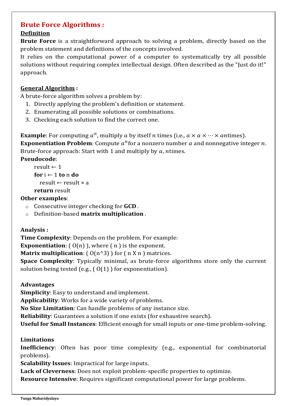
Brute Force Algorithms :
Definition
Brute Force is a straightforward approach to solving a problem, directly based on the
problem statement and definitions of the concepts involved.
It relies on the computational power of a computer to systematically try all possible
solutions without requiring complex intellectual design. Often described as the “Just do it!”
approach.
General Algorithm :
A brute-force algorithm solves a problem by:
1. Directly applying the problem’s definition or statement.
2. Enumerating all possible solutions or combinations.
3. Checking each solution to find the correct one.
Example: For computing 𝑎𝑛, multiply 𝑎 by itself 𝑛 times (i.e., 𝑎 × 𝑎 × ⋯ × 𝑎𝑛times).
Exponentiation Problem: Compute 𝑎𝑛for a nonzero number 𝑎 and nonnegative integer 𝑛.
Brute-force approach: Start with 1 and multiply by 𝑎, 𝑛times.
Pseudocode:
result ← 1
for i ← 1 to n do
result ← result × a
return result
Other examples:
o Consecutive integer checking for GCD .
o Definition-based matrix multiplication .
Analysis :
Time Complexity: Depends on the problem. For example:
Exponentiation: ( O(n) ), where ( n ) is the exponent.
Matrix multiplication: ( O(n^3) ) for ( n X n ) matrices.
Space Complexity : Typically minimal, as brute -force algorithms store only the current
solution being tested (e.g., ( O(1) ) for exponentiation).
Advantages
Simplicity: Easy to understand and implement.
Applicability: Works for a wide variety of problems.
No Size Limitation: Can handle problems of any instance size.
Reliability: Guarantees a solution if one exists (for exhaustive search).
Useful for Small Instances: Efficient enough for small inputs or one-time problem-solving.
Limitations
Inefficiency: Often has poor time complexity (e.g., exponential for combinatorial
problems).
Scalability Issues: Impractical for large inputs.
Lack of Cleverness: Does not exploit problem-specific properties to optimize.
Resource Intensive: Requires significant computational power for large problems.
Begin at result = 1. Each step performs one multiplication by a. At n = 0 the empty product is 1 and the multiplication count is zero.
Enable JavaScript for the animation. The complete notes and programs remain readable.
Added explanation · Python lab
The direct power algorithm has exactly n multiplications, so Θ(n) arithmetic-step time. It keeps a constant number of variables, but an arbitrary-precision result needs more bits as it grows. “No Size Limitation” in the source means the method is conceptually applicable; the limitations on the same page explain why exhaustive work may become practically infeasible. Direct definition-based algorithms do not all enumerate a combinatorial search space: matrix multiplication and exponentiation are brute-force examples too.
Brute-force exponentiation: multiply n timesmain.py
def brute_power(a, n):
result = 1
for i in range(n):
result *= a
return result, n
a, n = map(int, input().split())
if a == 0 or not 0 <= n <= 100:
raise ValueError("Use a nonzero base and an exponent from 0 to 100")
value, count = brute_power(a, n)
print("Power =", value)
print("Multiplications =", count)
Extra example named in the notes: consecutive-integer GCD starts at min(a,b) and checks descending candidates until one divides both inputs. For (12,18), candidates 12,11,10,9,8,7,6 give seven checks; 6 divides both. Euclid’s remainder method from Unit 1 usually needs far fewer arithmetic steps. This positive-input teaching version is kept separate from the source text.
Extra practice: consecutive-integer GCDmain.py
a, b = map(int, input().split())
if not 1 <= a <= 10000 or not 1 <= b <= 10000:
raise ValueError("Use positive integers up to 10000")
candidate = min(a, b)
candidates = 0
while candidate >= 1:
candidates += 1
if a % candidate == 0 and b % candidate == 0:
break
candidate -= 1
print("GCD =", candidate)
print("Candidates checked =", candidates)
Tunga Mahavidyalaya
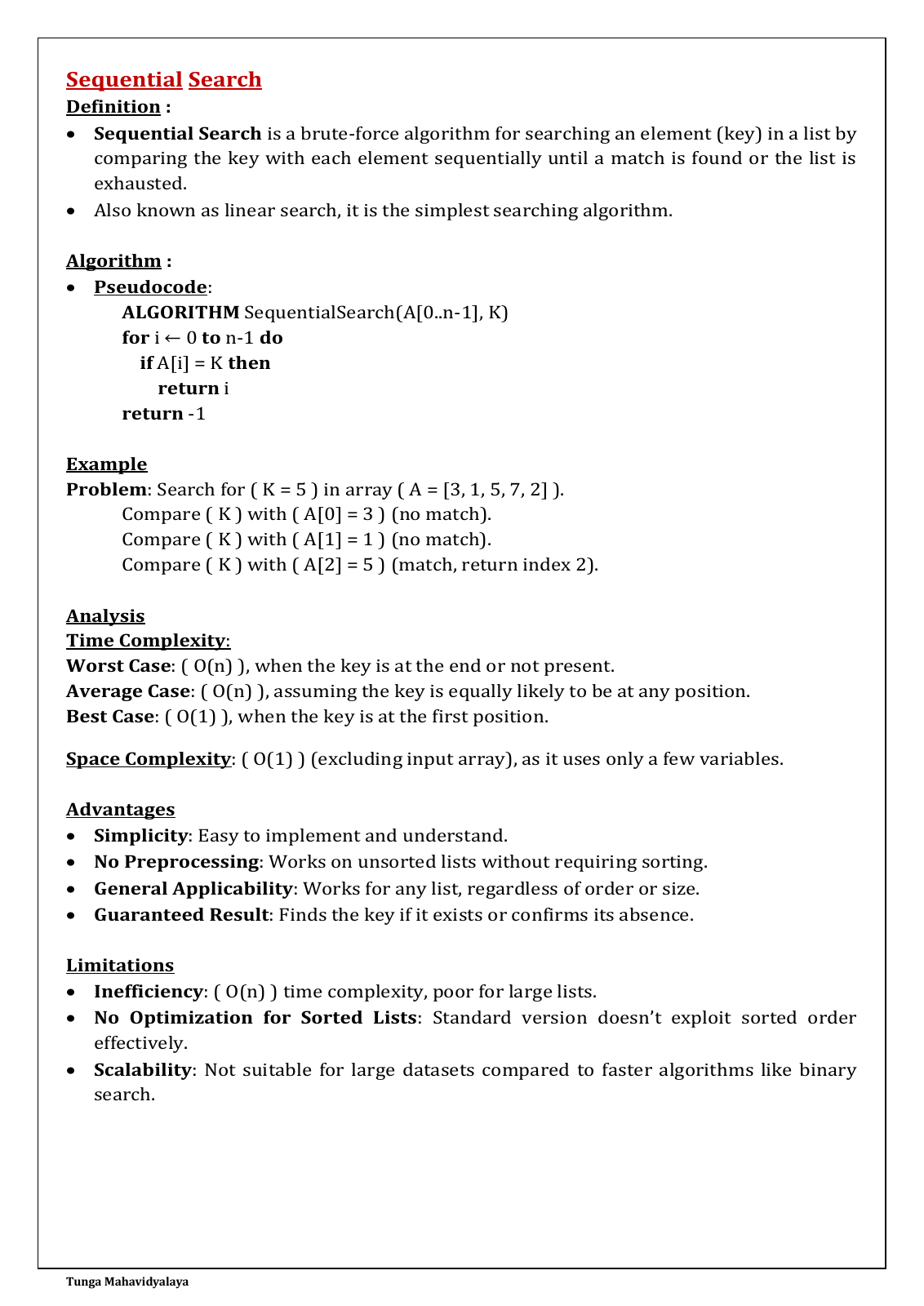
Sequential Search
Definition :
• Sequential Search is a brute-force algorithm for searching an element (key) in a list by
comparing the key with each element sequentially until a match is found or the list is
exhausted.
• Also known as linear search, it is the simplest searching algorithm.
Algorithm :
• Pseudocode:
ALGORITHM SequentialSearch(A[0..n-1], K)
for i ← 0 to n-1 do
if A[i] = K then
return i
return -1
Example
Problem: Search for ( K = 5 ) in array ( A = [3, 1, 5, 7, 2] ).
Compare ( K ) with ( A[0] = 3 ) (no match).
Compare ( K ) with ( A[1] = 1 ) (no match).
Compare ( K ) with ( A[2] = 5 ) (match, return index 2).
Analysis
Time Complexity:
Worst Case: ( O(n) ), when the key is at the end or not present.
Average Case: ( O(n) ), assuming the key is equally likely to be at any position.
Best Case: ( O(1) ), when the key is at the first position.
Space Complexity: ( O(1) ) (excluding input array), as it uses only a few variables.
Advantages
• Simplicity: Easy to implement and understand.
• No Preprocessing: Works on unsorted lists without requiring sorting.
• General Applicability: Works for any list, regardless of order or size.
• Guaranteed Result: Finds the key if it exists or confirms its absence.
Limitations
• Inefficiency: ( O(n) ) time complexity, poor for large lists.
• No Optimization for Sorted Lists : Standard version doesn’t exploit sorted order
effectively.
• Scalability: Not suitable for large datasets compared to faster algorithms like binary
search.
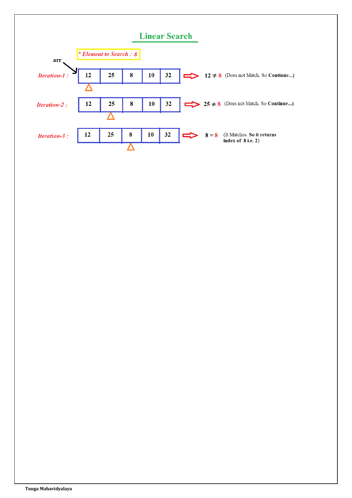
Linear Search
* Element to Search : 8
arr = [12, 25, 8, 10, 32]
Iteration - 1: compare index 0. 12 ≠ 8 (Does not Match. So Continue...)
Iteration - 2: compare index 1. 25 ≠ 8 (Does not Match. So Continue...)
Iteration - 3: compare index 2. 8 = 8 (It Matches. So it returns index of 8 i.e. 2)
The returned position is a zero-based index. A duplicate key returns its first matching index. Try an absent key to inspect every element and return −1.
Enable JavaScript for the animation. The complete notes and programs remain readable.
Added explanation · Python lab
Page 11 finds 5 at index 2 after three comparisons. Page 12 finds 8 at index 2 after three comparisons. For n ≥ 1 the best comparison count is 1, the worst is n, and a successful uniformly distributed first-match position gives (n + 1)/2 on average. If failure is possible, include its probability: p(n + 1)/2 + (1 − p)n under that same successful-position model. No sorting is required. Binary search requires sorted random-access data and is a different algorithm.
Sequential search: the example from your notesmain.py
def sequential_search(values, key):
comparisons = 0
for i in range(len(values)):
comparisons += 1
if values[i] == key:
return i, comparisons
return -1, comparisons
values = list(map(int, input().split()))
key = int(input())
index, comparisons = sequential_search(values, key)
print("Index =", index)
print("Comparisons =", comparisons)
Comparison: best 1, worst n; uniform success (n + 1)/2
Best Θ(1), worst/average Θ(n)
Θ(1) auxiliary
Added explanation · Python lab
State the chosen model. Fixed-size array element comparisons are treated as constant-time here. Large Python integers make multiplication cost depend on operand length. Input parsing and displaying results are additional program work; counters in these examples measure the selected algorithm operation. The PDF’s asymptotic claims and derivations are preserved above, with these assumptions added for practice.
DAA · UNIT 2 · 09
Run the algorithm. Change the input.
Choose an example and load it into the embedded Python interpreter. Select I/O inside the compiler, check the sample STDIN, and press Run. Change the input or edit the source to explore a different case.
Sample input (STDIN)
7 2 9 4
Expected output
Maximum = 9
Comparisons = 3
Load the compiler when you’re ready to practise.
>_
Your Python workspace
Edit real Python code and see real compiler output.
Compiler provided by OneCompiler. Opening the editor connects to that service; code and input you run are processed there. If the embed is unavailable, open the Python playground in a new tab and paste the source below.
View / copy the selected source
def max_element(values):
if not values:
raise ValueError("The array must be nonempty")
maximum, comparisons = values[0], 0
for i in range(1, len(values)):
comparisons += 1
if values[i] > maximum:
maximum = values[i]
return maximum, comparisons
values = list(map(int, input().split()))
maximum, comparisons = max_element(values)
print("Maximum =", maximum)
print("Comparisons =", comparisons)
All eight examples use Python 3. The array programs accept one line of integers. Search reads the key on a second line. Matrix input is its order n, then n rows of A, then n rows of B. The selected sample input shows the complete format. Counting variables are included for learning; the source algorithms are retained in the notes above.
For each algorithm, state its input size, basic operation, case, sum or recurrence, initial condition when needed, and final growth class. Keep exact counts and asymptotic notation distinct.